Traffic Sign Classification
December 30, 2018
Having just finished the semester at NYU, I thought I’d share the results of one of the more interesting homework assignments that I had. As the title suggests, this will be another post about the traffic sign classification competition found at http://benchmark.ini.rub.de/.
For some background, I am currently studying for my master’s degree at NYU. Like many of the other students there, I jumped at the chance to take the computer vision class taught by the renowned professor Rob Fergus.
Cool, but what makes this assignment more interesting than any other assignment from any other professor? This homework assignment was given in the form of a Kaggle competition. The higher your rank on the private leaderboard the higher your grade.
For those that don’t know what the private leaderboard is on Kaggle, there are two different leaderboards in a Kaggle competition. The public leaderboard and the private leaderboard. While the competition is active, all submissions are shown on the public leaderboard. This ranking is based on your score from 50% of the test data. When the competition ends, your score is calculated from the other 50% of the test data to rank you on the private leaderboard. Obviously, you are not told what data is used on which leaderboard. This is to prevent you from over-fitting the test data.
The requirement to get a passing grade at all was to get at least 90% accuracy on the test data. To achieve this milestone, I started with a simple convolutional neural network and a naively chosen validation set. Each traffic sign had different images taken in varying positions with a varying amount of light. I took the first three types of images for each traffic sign and moved them to a different directory to use as the validation set.
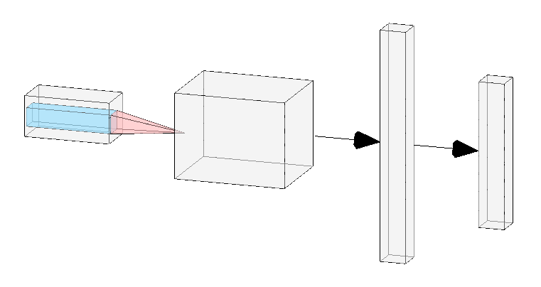
Representation of CNN architecture used. 2 conv layers followed by 2 linear layers. Not sure how people draw their beautiful network architecture diagrams…
nclasses = 43

class BaseNet(nn.Module):
    def __init__(self):
        super(BaseNet, self).__init__()
        self.conv1 = nn.Conv2d(3, 10, kernel_size=5)
        self.conv2 = nn.Conv2d(10, 20, kernel_size=5)
        self.conv2_drop = nn.Dropout2d()

        self.fc1 = nn.Linear(500, 50)
        self.fc2 = nn.Linear(50, nclasses)

    def forward(self, x):
        x = F.relu(F.max_pool2d(self.conv1(x), 2))
        x = F.relu(F.max_pool2d(self.conv2_drop(self.conv2(x)), 2))

        x = x.view(-1, 500)
        x = F.relu(self.fc1(x))
        x = F.dropout(x, training=self.training)

        x = self.fc2(x)
        return F.log_softmax(x)
The first network consisted of 2 convolution layers followed by 2 linear layers. I used a step scheduler to decay the learning rate by 0.1 after every 5 epochs. This simple model was surprisingly able to achieve 89% accuracy after 25 epochs.
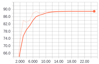
Validation accuracy values after running for 25 epochs.
Unfortunately, training this model for more epochs did not look like it would do any good since we can see from the graph of the validation loss values that the loss values have plateaued.
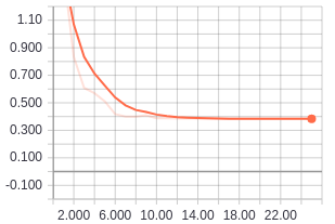
Validation losses for a 25 epoch run on the simple CNN model.
Since this was just shy of the 90% accuracy goal, I thought why not add a few more convolution layers and another linear layer. Heck, lets throw in some batch normalization and dropout layers to prevent any over-fitting problems this early in the game.
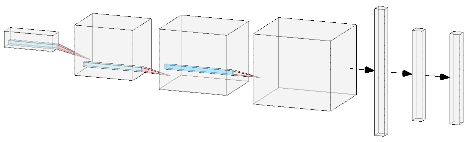
New CNN model with batch normalization and dropouts added between conv layers.
I added 2 more conv layers and 1 more linear layer. I also added batch normalization and dropout after the second and fourth conv layers. Batch normalization was also inserted after the first and second linear layers.
nclasses = 43

class DeepNet(nn.Module):
    def __init__(self):
        super(DeepNet, self).__init__()
        self.conv1 = nn.Conv2d(3, 32, kernel_size=3)
        self.conv2 = nn.Conv2d(32, 64, kernel_size=3)
        self.conv_bn1 = nn.BatchNorm2d(64)
        self.conv2_drop = nn.Dropout2d()

        self.conv3 = nn.Conv2d(64, 128, kernel_size=3)
        self.conv4 = nn.Conv2d(128, 256, kernel_size=3)
        self.conv_bn2 = nn.BatchNorm2d(256)
        self.conv4_drop = nn.Dropout2d()

        self.fc1 = nn.Linear(6400, 512)
        self.fc1_bn = nn.BatchNorm1d(512)

        self.fc2 = nn.Linear(512, 512)
        self.fc2_bn = nn.BatchNorm1d(512)

        self.fc3 = nn.Linear(512, nclasses)

    def forward(self, x):
        x = self.conv1(x)
        x = F.relu(F.max_pool2d(
                  self.conv2_drop(self.conv_bn1(self.conv2(x))), 2))

        x = self.conv3(x)
        x = F.relu(F.max_pool2d(self.conv4_drop(
                                self.conv_bn2(self.conv4(x))), 2))

        x = x.view(-1, self.num_flat_features(x))

        x = F.relu(self.fc1_bn(self.fc1(x)))
        x = F.dropout(x, training=self.training)

        x = F.relu(self.fc2_bn(self.fc2(x)))
        x = F.dropout(x, training=self.training)

        x = self.fc3(x)
        return F.log_softmax(x)

    def num_flat_features(self, x):
        size = x.size()[1:]
        num_features = 1
        for s in size:
            num_features *= s
        return num_features
Running this model for 25 epochs then put me at 96% validation accuracy! This was just a model consisting of a bunch of convolutional and linear layers smashed together. It should make you wonder about the performance that can be achieved on networks that have been shown to perform well on much more complicated datasets like ImageNet.
Validation accuracy after 25 epochs with deeper CNN.
It was now time to pull out the big guns. Since I was able to hit 96% accuracy with such a simple network, I did not believe it was necessary to use something like ResNet152. In fact, I am pretty sure a network of that size would have serious problems with over-fitting. I opted for the smaller ResNet18.
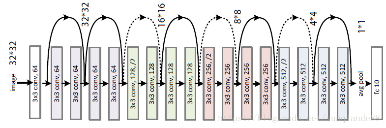
ResNet18, image found on Google images.
nclasses = 43

class ResNet(nn.Module):
    def __init__(self):
        super(ResNet, self).__init__()
        self.resnet = resnet18()
        self.resnet.fc = nn.Linear(512, nclasses)

    def forward(self, x):
        x = self.resnet(x)
        return F.log_softmax(x)
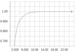
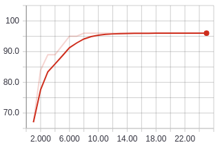
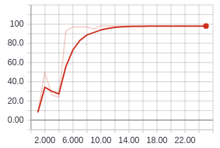
Training accuracy using ResNet18.
Validation accuracy using ResNet18.
This put me at 98% validation accuracy with 3798 traffic signs classified correctly out of 3870 after running for 25 epochs. As we can see from the graphs, the training accuracy is at 100% so we will probably not get any more accuracy out of this model even if we ran it for more epochs.
Since the training accuracy was at 100%, it was safe to assume that the model was over-fitting the training set and so not achieving a higher validation accuracy. At this point, it made sense to take a look at some of the images that the model classified incorrectly.
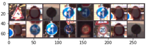
Incorrectly classified images in the validation set.
The images that the model struggled with the most were the images that had bad or inconsistent lighting. I decided to use ColorJittering to randomize the brightness in the training images. Some of the incorrectly classified images also looked like they were off center so I also used RandomAffine to add random rotations, scaling and translations into the training images. This led me to use the following transformations for data augmentation:
data_transforms = transforms.Compose([
    transforms.Resize((224, 224)),
    transforms.ColorJitter(0.8, contrast=0.4),
    transforms.RandomAffine(15,
                            scale=(0.8, 1.2),
                            translate=(0.2, 0.2)),
    transforms.ToTensor(),
    transforms.Normalize((0.3337, 0.3064, 0.3171),
                         (0.2672, 0.2564, 0.2629))
])

validation_data_transforms = transforms.Compose([
    transforms.Resize((224, 224)),
    transforms.ToTensor(),
    transforms.Normalize((0.3337, 0.3064, 0.3171),
                         (0.2672, 0.2564, 0.2629))
])
Notice that I do not perform the random transforms on the validation images. We perform the transformations during training to create different randomized variations of the training images. This has the effect of increasing our training set size and hence helping us to fight over-fitting. We do not want to make it more difficult for our model during validation to classify the validation images.
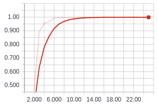
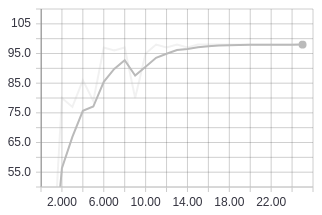
Training accuracy using ResNet18 with data augmentation.
Validation accuracy using ResNet18 with data augmentation.
The validation accuracy comes in at 98% again, although this time it is able to get a few more images classified correctly. This model was able to classify 3818 traffic signs correctly out of 3870. To get the final model for submission, I combined the training and validation sets to get even more training data. I loaded up the model parameters of the model that was able to correctly classify 3818 images and I trained for 3 more epochs. Submitting this final model gave me a score of 0.99283. Not too bad.
The repository containing the models and the script to run training can be found at https://github.com/AaronCCWong/german-traffic-sign-recognition.