Building a Bigram Hidden Markov Model for Part-Of-Speech Tagging

May 18, 2019

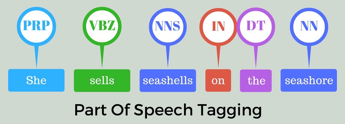
Image credits: Google Images

Links to an example implementation can be found at the bottom of this post.

Part-of-Speech tagging is an important part of many natural language processing pipelines where the words in a sentence are marked with their respective parts of speech. An example application of part-of-speech (POS) tagging is chunking. Chunking is the process of marking multiple words in a sentence to combine them into larger “chunks”. These chunks can then later be used for tasks such as named-entity recognition. Let’s explore POS tagging in depth and look at how to build a system for POS tagging using hidden Markov models and the Viterbi decoding algorithm.

What are the POS tags?

There are 9 main parts of speech as can be seen in the following figure.

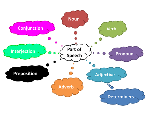
Image credits: Google Images

The POS tags used in most NLP applications are more granular than this. An example of this is NN and NNS where NN is used for singular nouns such as “table” while NNS is used for plural nouns such as “tables”. The most prominent tagset is the Penn Treebank tagset consisting of 36 POS tags.

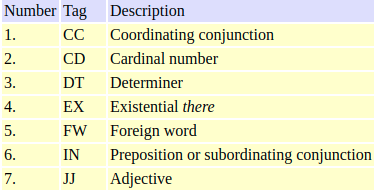
Subset of the Penn Treebank tagset

The full Penn Treebank tagset can be found here.

Hidden Markov Models

Luckily for us, we don’t have to perform POS tagging by hand. We will instead use hidden Markov models for POS tagging.

For those of us that have never heard of hidden Markov models (HMMs), HMMs are Markov models with hidden states. So what are Markov models and what do we mean by hidden states? A Markov model is a stochastic (probabilistic) model used to represent a system where future states depend only on the current state. For the purposes of POS tagging, we make the simplifying assumption that we can represent the Markov model using a finite state transition network.

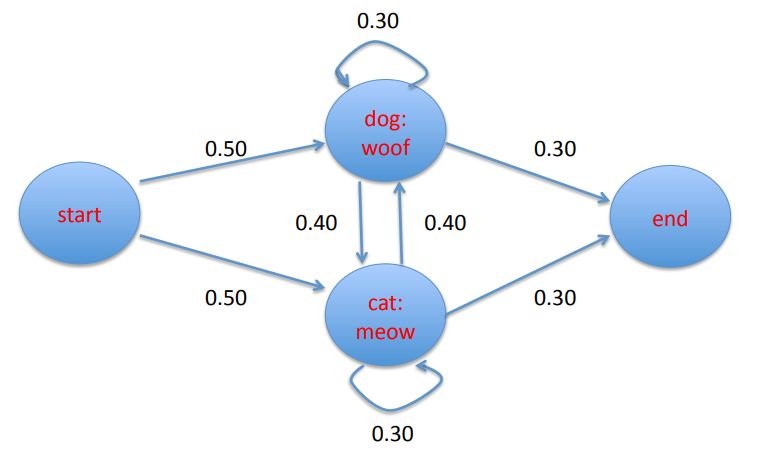
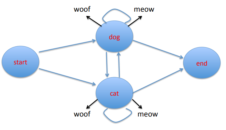
A finite state transition network representing a Markov model. Image credits: Professor Ralph Grishman at NYU.

Each of the nodes in the finite state transition network represents a state and each of the directed edges leaving the nodes represents a possible transition from that state to another state. Note that each edge is labeled with a number representing the probability that a given transition will happen at the current state. Note also that the probability of transitions out of any given state always sums to 1.

In the finite state transition network pictured above, each state was observable. We are able to see how often a cat meows after a dog woofs. What if our cat and dog were bilingual. That is, what if both the cat and the dog can meow and woof? Furthermore, let’s assume that we are given the states of dog and cat and we want to predict the sequence of meows and woofs from the states. In this case, we can only observe the dog and the cat but we need to predict the unobserved meows and woofs that follow. The meows and woofs are the hidden states.

A finite state transition network representing an HMM. Image credits: Professor Ralph Grishman at NYU.

The figure above is a finite state transition network that represents our HMM. The black arrows represent emissions of the unobserved states woof and meow.

Let’s now take a look at how we can calculate the transition and emission probabilities of our states. Going back to the cat and dog example, suppose we observed the following two state sequences:

dog, cat, cat
dog, dog, dog

Then the transition probabilities can be calculated using the maximum likelihood estimate:

\[P(s_{i} \vert s_{i-1}) = \frac{C(s_{i}, s_{i-1})}{C(s_{i-1})}\]

In English, this says that the transition probability from state i-1 to state i is given by the total number of times we observe state i-1 transitioning to state i divided by the total number of times we observe state i-1.

For example, from the state sequences we can see that the sequences always start with dog. Thus we are at the start state twice and both times we get to dog and never cat. Hence the transition probability from the start state to dog is 1 and from the start state to cat is 0.

Let’s try one more. Let’s calculate the transition probability of going from the state dog to the state end. From our example state sequences, we see that dog only transitions to the end state once. We also see that there are four observed instances of dog. Thus the transition probability of going from the dog state to the end state is 0.25. The other transition probabilities can be calculated in a similar fashion.

The emission probabilities can also be calculated using maximum likelihood estimates:

\[P(t_{i} \vert s_{i}) = \frac{C(t_{i}, s_{i})}{C(s_{i})}\]

In English, this says that the emission probability of tag i given state i is the total number of times we observe state i emitting tag i divided by the total number of times we observe state i.

Let’s calculate the emission probability of dog emitting woof given the following emissions for our two state sequences above:

woof, woof, meow
meow, woof, woof

That is, for the first state sequence, dog woofs then cat woofs and finally cat meows. We see from the state sequences that dog is observed four times and we can see from the emissions that dog woofs three times. Thus the emission probability of woof given that we are in the dog state is 0.75. The other emission probabilities can be calculated in the same way. For completeness, the completed finite state transition network is given here:

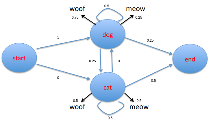
Finite state transition network of the hidden Markov model of our example.

So how do we use HMMs for POS tagging? When we are performing POS tagging, our goal is to find the sequence of tags T such that given a sequence of words W we get

\[T = \text{argmax}_{\hat{T}} P(\hat{T} \vert W)\]

In English, we are saying that we want to find the sequence of POS tags with the highest probability given a sequence of words. As tag emissions are unobserved in our hidden Markov model, we apply Baye’s rule to change this probability to an equation we can compute using maximum likelihood estimates:

\[T = \text{argmax}_{\hat{T}} P(\hat{T} \vert W) = \text{argmax}_{\hat{T}} \frac{P(W \vert \hat{T}) P(\hat{T})}{P(W)} \propto \text{argmax}_{\hat{T}} P(W \vert \hat{T}) P(\hat{T})\]

The second equals is where we apply Baye’s rule. The symbol that looks like an infinity symbol with a piece chopped off means proportional to. This is because $P(W)$ is a constant for our purposes since changing the sequence T does not change the probability $P(W)$. Thus dropping it will not make a difference in the final sequence T that maximizes the probability.

In English, the probability $P(W \vert T)$ is the probability that we get the sequence of words given the sequence of tags. To be able to calculate this we still need to make a simplifying assumption. We need to assume that the probability of a word appearing depends only on its own tag and not on context. That is, the word does not depend on neighboring tags and words. Then we have

\[P(W \vert \hat{T}) \approx \Pi_{i=1}^{n} P(w_{i} \vert \hat{t}_{i})\]

In English, the probability $P(T)$ is the probability of getting the sequence of tags T. To calculate this probability we also need to make a simplifying assumption. This assumption gives our bigram HMM its name and so it is often called the bigram assumption. We must assume that the probability of getting a tag depends only on the previous tag and no other tags. Then we can calculate $P(T)$ as

\[P(\hat{T}) \approx \Pi_{i=1}^{n} P(\hat{t}_{i} \vert \hat{t}_{i-1})\]

Note that we could use the trigram assumption, that is that a given tag depends on the two tags that came before it. As it turns out, calculating trigram probabilities for the HMM requires a lot more work than calculating bigram probabilities due to the smoothing required. Trigram models do yield some performance benefits over bigram models but for simplicity’s sake we use the bigram assumption.

Finally, we are now able to find the best tag sequence using

\[T \approx \text{argmax}_{\hat{T}} \Pi_{i=1}^{n} P(w_{i} \vert \hat{t}_{i}) P(\hat{t}_{i} \vert \hat{t}_{i-1})\]

The probabilities in this equation should look familiar since

\[P(w_{i} \vert \hat{t}_{i})\]

is the emission probability and

\[P(\hat{t}_{i} \vert \hat{t}_{i-1})\]

is the transition probability.

Hence if we were to draw a finite state transition network for this HMM, the observed states would be the tags and the words would be the emitted states similar to our woof and meow example. We have already seen that we can use the maximum likelihood estimates to calculate these probabilities.

Given a dataset consisting of sentences that are tagged with their corresponding POS tags, training the HMM is as easy as calculating the emission and transition probabilities as described above. For an example implementation, check out the bigram model as implemented here. The basic idea of this implementation is that it primarily keeps count of the values required for maximum likelihood estimation during training. The model then calculates the probabilities on the fly during evaluation using the counts collected during training.

An astute reader would wonder what the model does in the face of words it did not see during training. We return to this topic of handling unknown words later as we will see that it is vital to the performance of the model to be able to handle unknown words properly.

Viterbi Decoding

Image credits: Google Images

The HMM gives us probabilities but what we want is the actual sequence of tags. We need an algorithm that can give us the tag sequence with highest probability of being correct given a sequence of words. An intuitive algorithm for doing this, known as greedy decoding, goes and chooses the tag with the highest probability for each word without considering context such as subsequent tags. As we know, greedy algorithms don’t always return the optimal solution and indeed it returns a sub-optimal solution in the case of POS tagging. This is because after a tag is chosen for the current word, the possible tags for the next word may be limited and sub-optimal leading to an overall sub-optimal solution.

We instead use the dynamic programming algorithm called Viterbi. Viterbi starts by creating two tables. The first table is used to keep track of the maximum sequence probability that it takes to reach a given cell. If this doesn’t make sense yet that is okay. We will take a look at an example. The second table is used to keep track of the actual path that led to the probability in a given cell in the first table.

Let’s look at an example to help this settle in. Returning to our previous woof and meow example, given the sequence

meow woof

we will use Viterbi to find the most likely sequence of states that led to this sequence. First we need to create our first Viterbi table. We need a row for every state in our finite state transition network. Thus our table has 4 rows for the states start, dog, cat and end. We are trying to decode a sequence of length two so we need four columns. In general, the number of columns we need is the length of the sequence we are trying to decode. The reason we need four columns is because the full sequence we are trying to decode is actually

<start> meow woof <woof>

The first table consists of the probabilities of getting to a given state from previous states. Let $a_{ij}$ be the transition probability from state $s_{i}$ to $s_{j}$ and $b_{jt}$ be the emission probability of the word $w_{t}$ at state $s_{j}$. Then more precisely, the value of each cell is given by

\[v_{t}(j) = \max_{i=1}^{n} v_{t-1}(i) a_{ij} b_{jt}\]

Let’s fill out the table for our example using the probabilities we calculated for the finite state transition network of the HMM model.

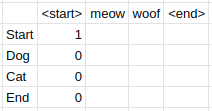
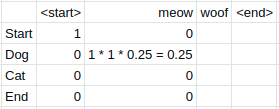
Notice that the first column has 0 everywhere except for the start row. This is because the sequences for our example always start with . From our finite state transition network, we see that the start state transitions to the dog state with probability 1 and never goes to the cat state. We also see that dog emits meow with a probability of 0.25\. It is also important to note that we cannot get to the start state or end state from the start state. Thus we get the next column of values

Notice that the probabilities of all the states we can’t get to from our start state are 0. Also, the probability of getting to the dog state for the meow column is 1 * 1 * 0.25 where the first 1 is the previous cell’s probability, the second 1 is the transition probability from the previous state to the dog state and 0.25 is the emission probability of meow from the current state dog. Thus 0.25 is the maximum sequence probability so far. Continuing onto the next column:

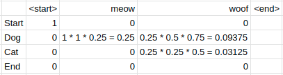
Observe that we cannot get to the start state from the dog state and the end state never emits woof so both of these rows get 0 probability. Meanwhile, the cells for the dog and cat state get the probabilities 0.09375 and 0.03125 calculated in the same way as we saw before with the previous cell’s probability of 0.25 multiplied by the respective transition and emission probabilities. Finally, we get

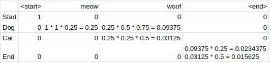
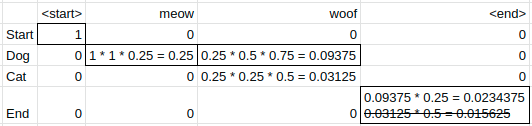
At this point, both cat and dog can get to . Thus we must calculate the probabilities of getting to end from both cat and dog and then take the path with higher probability.

Going from dog to end has a higher probability than going from cat to end so that is the path we take. Thus the answer we get should be

<start> dog dog <end>

In a Viterbi implementation, the whole time we are filling out the probability table another table known as the backpointer table should also be filled out. The value of each cell in the backpointer table is equal to the row index of the previous state that led to the maximum probability of the current state. Thus in our example, the end state cell in the backpointer table will have the value of 1 (0 starting index) since the state dog at row 1 is the previous state that gave the end state the highest probability. For completeness, the backpointer table for our example is given below.

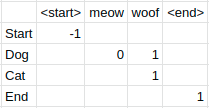
Note that the start state has a value of -1. This is the stopping condition we use for when we trace the backpointer table backwards to get the path that provides us the sequence with the highest probability of being correct given our HMM. To get the state sequence dog dog , we start at the end cell on the bottom right of the table. The 1 in this cell tells us that the previous state in the woof column is at row 1 hence the previous state must be dog. From dog, we see that the cell is labeled 1 again so the previous state in the meow column before dog is also dog. Finally, in the meow column, we see that the dog cell is labeled 0 so the previous state must be row 0 which is the state. We see -1 so we stop here. Our sequence is then dog dog . Reversing this gives us our most likely sequence.

Check out an example implementation of Viterbi here.

When using an algorithm, it is always good to know the algorithmic complexity of the algorithm. In the case of Viterbi, the time complexity is equal to $O(s^{2}n)$ where $s$ is the number of states and $n$ is the number of words in the input sequence. This is because for each of the $sn$ entries in the probability table, we need to look at the s entries in the previous column. The space complexity required is $O(sn)$. This is because there are $s$ rows, one for each state, and $n$ columns, one for each word in the input sequence.

Performance Evaluation

Let’s see what happens when we try to train the HMM on the WSJ corpus. I have not been given permission to share the corpus so cannot point you to one here but if you look for it, it shouldn’t be hard to find…

Training the HMM and then using Viterbi for decoding gets us an accuracy of 71.66% on the validation set. Meanwhile the current benchmark score is 97.85%.

Handling Unknown Words

How can we close this gap? We already know that using a trigram model can lead to improvements but the largest improvement will come from handling unknown words properly. We use the approach taken by Brants in the paper TnT — A Statistical Part-Of-Speech Tagger. More specifically, we perform suffix analysis to attempt to guess the correct tag for an unknown word.

We create two suffix trees. One suffix tree to keep track of the suffixes of lower cased words and one suffix tree to keep track of the suffixes of upper cased words. (Brants, 2000) found that using different probability estimates for upper cased words and lower cased words had a positive effect on performance. This makes sense since capitalized words are more likely to be things such as acronyms.

We use only the suffixes of words that appear in the corpus with a frequency less than some specified threshold. The maximum suffix length to use is also a hyperparameter that can be tuned. Empirically, the tagger implementation here was found to perform best when a maximum suffix length of 5 and maximum word frequency of 25 was used giving a tagging accuracy of 95.79% on the validation set.

To calculate the probability of a tag given a word suffix, we follow (Brants, 2000) and use

\[P(t \vert l_{n-i+1},...,l_{n}) = \frac{\hat{P}(t \vert l_{n-i+1},...,l_{n}) + \theta P(t \vert l_{n-i},...,l_{n})}{1 + \theta}\]

where

\[\hat{P}(t \vert l_{n-i+1},...,l_{n})\]

is calculated using the maximum likelihood estimate like we did in previous examples and

\[\theta = \frac{1}{s-1} \sum_{i=1}^{s} \left( \hat{P}(t_{i}) - \bar{P} \right)^{2}\]

where

\[\bar{P} = \frac{1}{s} \sum_{j=1}^{s} \hat{P}(t_{j}).\]

In English, the probability of a tag given a suffix is equal to the smoothed and normalized sum of the maximum likelihood estimates of all the suffixes of the given suffix.

Thus, during the calculation of the Viterbi probabilities, if we come across a word that the HMM has not seen before we can consult our suffix trees with the suffix of the unknown word. Instead of calculating the emission probabilities of the tags of the word with the HMM, we use the suffix tree to calculate the emission probabilities of the tags given the suffix of the unknown word.

To see an example implementation of the suffix trees, check out the code here. As already stated, this raised our accuracy on the validation set from 71.66% to 95.79%.